Do read this: article by BCG predicting the economic impact of quantum computing in the NISQ era and beyond - which estimates the economic impact of quantum computing in the next 5 years to be $2 - 5 billion.

My inner quantum physicist sprung into action and I decided to make a tangible application on a quantum computer - however simple it maybe.

All code can be found at this repository

So What’s Happening Exactly ?

First things first - what am I trying here ? - basically I am trying to build a frequency detector on a quantum computer, audio file goes in and most dominant frequencies come out, thats it. (some might ask - aren’t you making a glorified version of a quantum version of discrete fourier transform ? -> well yeh but sshhh!). I plan to start with simple audio signal of a pure sine wave. If things work out I may try to record a note played on a guitar.

TLDR; - I want to make a frequency detector using a quantum computer

Why should I care ?

Apart from having the potential to crack your facebook/instagram/bank account passwords, QFT or Fourier transform is one of the central tools in mathematics and is used almost in every piece of tech that you see around you in some way. The difference between Quantum Fourier Transform and classical Fast Fourier transform is in the speed and in the way the data is represented physically. Classically, a dimension $n$ vector would need $n$ floating point numbers. On a quantum computer, the QFT operates on the wave function needing only $log_{2}(n)$ qubits, exponentially saving space. The best classical FFT runs in time $O(n log(n))$ and the QFT runs in time $O(log(n)^{2})$ where again $n$ is the dimension of the vector. Also the classical FFT must take time $O(n)$ to even read the input!

The vanilla QFT algorithm takes $O(n^{2})$ quantum gates, but there are very efficient approximate versions which need only $O(n log(n))$ gates possibly giving more speedup.

1. Quantum Fourier Transform

QFT is the quantum version of the discrete fourier transform. In QFT we encode the input vector as a set of amplitudes of the basis states of the quantum system. Hence, the number of points we can operate over is restricted by the number of qubits available to us.

The classical fourier transform acts on a vector $(x_{0}, x_{1},...,x_{N-1})$ and calculates $(y_{0}, y_{1},...,y_{N-1})$ where

$\large y_{k} = \frac{1}{\sqrt{N}}\sum_{i=0}^{N-1}x_{i}\omega_{N}^{-ik}$

where $\omega_{N}=e^{\frac{2\pi i}{N}}$

The quantum fourier transform does something similar. It acts on a quantum state

$\large |x\rangle = \sum_{i=0}^{N-1}x_{i}|i\rangle$

and maps it to a quantum state

$\large |y\rangle =\sum_{i=0}^{N-1}y_{i}|i\rangle$

according to the equation:

$\large y_{k} = \frac{1}{\sqrt{N}}\sum_{i=0}^{N-1}x_{i}\omega_{N}^{ik},\;\;\;\;\; k = 0,1,2,..., N-1$

I am using the convention which makes the QFT have the same effect as the inverse discrete fourier transform. Depending on the implementation of the circuit this convention can change.

If we deal with basis states then QFT can also be expressed as a map:

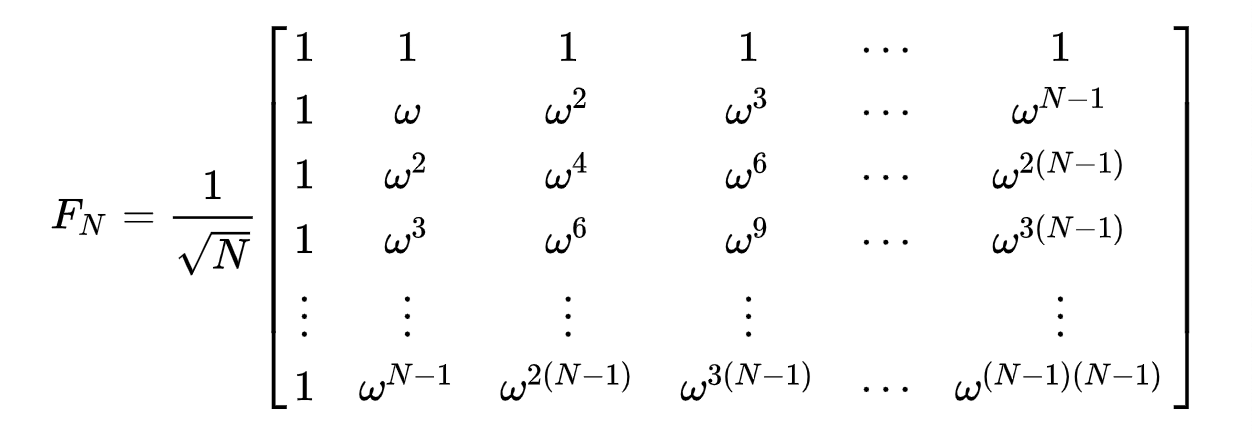
$\large QFT |x\rangle = \frac{1}{\sqrt{N}}\sum_{k=0}^{N-1}\omega_{N}^{xk}|k\rangle,\;\;\;\;\; k = 0,1,2,..., N-1$

If you are the sort of person who better understands stuff in terms of unitaries, the equivalent unitary for QFT is

QFT Unitary

1.1 Building the quantum circuit for QFT

* Quirk visualizer by Craig Gidney

The quantum processors that we currently have encode operations in quantum gates. The next few lines rewrite the QFT equation into a form which can be implemented as a quantum circuit using the commonly available quantum gates. You can skip this if you want.

$\large QFT |x\rangle = \frac{1}{\sqrt{N}}\sum_{k=0}^{2^{n}-1}\omega_{N}^{xk}|k\rangle = \frac{1}{\sqrt{N}}\sum_{k_{1}\in \{0,1\}}\sum_{k_{2}\in \{0,1\}}\sum_{k_{3}\in \{0,1\}}\text{...}\sum_{k_{n}\in \{0,1\}}\omega_{N}^{x\sum_{j=1}^{n}k_{j}2^{n-j}}|k_{1}k_{2}k_{3}...k_{n}\rangle$

1.2 Digression

To understand the above equation it would help to expand it using a small n. For example for a 2 qubit system, the basis states are

$\large |00\rangle, |01\rangle, |10\rangle, |11\rangle$ $\large QFT |x\rangle = \frac{1}{\sqrt{4}}\sum_{k_{1}\in\{0,1\}}\sum_{k_{2}\in\{0,1\}}\omega_{4}^{x\sum_{j=1}^{2}k_{j}2^{2-j}}|k_{1},k_{2}\rangle$

1.3 Moving on

Hence,

$\large QFT|x\rangle = \frac{1}{\sqrt{N}}\sum_{k_{1}\in \{0,1\}}\sum_{k_{2}\in \{0,1\}}\sum_{k_{3}\in \{0,1\}}\text{...}\sum_{k_{n}\in \{0,1\}} \bigotimes_{j=1}^{n}\omega_{N}^{xk_{j}2^{n-j}}|k_{j}\rangle$ $\large = \frac{1}{\sqrt{N}}\sum_{k_{1}\in \{0,1\}}\sum_{k_{2}\in \{0,1\}}\sum_{k_{3}\in \{0,1\}}\text{...}\sum_{k_{n}\in \{0,1\}}\omega_{N}^{xk_{1}2^{n-1}}|k_{1}\rangle\otimes \bigotimes_{j=2}^{n}\omega_{N}^{xk_{j}2^{n-j}}|k_{j}\rangle$ $\large = \frac{1}{\sqrt{N}}\left(\sum_{k_{1}\in\{0,1\}}\omega_{N}^{xk_{1}2^{n-1}}|k_1\rangle\right)\otimes\left(\sum_{k_{2}\in\{0,1\}}\omega_{N}^{xk_{2}2^{n-2}}|k_2\rangle\right)\otimes\sum_{k_{3}\in \{0,1\}}\text{...}\sum_{k_{n}\in \{0,1\}}\omega_{N}^{xk_{3}2^{n-3}}|k_3\rangle\otimes\bigotimes_{j=3}^{n}\omega_{N}^{xk_{j}2^{n-j}}|k_{j}\rangle$ $\large = \frac{1}{\sqrt{N}}\left(\sum_{k_{1}\in\{0,1\}}\omega_{N}^{xk_{1}2^{n-1}}|k_1\rangle\right)\otimes\left(\sum_{k_{2}\in\{0,1\}}\omega_{N}^{xk_{2}2^{n-2}}|k_2\rangle\right)\otimes\left(\sum_{k_{3}\in\{0,1\}}\omega_{N}^{xk_{3}2^{n-3}}|k_3\rangle\right)\otimes\sum_{k_{4}\in \{0,1\}}\text{...}\sum_{k_{n}\in \{0,1\}}\omega_{N}^{xk_{4}2^{n-4}}|k_4\rangle\otimes\bigotimes_{j=4}^{n}\omega_{N}^{xk_{j}2^{n-j}}|k_{j}\rangle$

Hence, the original QFT equation can be rewritten in terms of individual qubits as :

$\large = \frac{1}{\sqrt{N}}\bigotimes_{j=1}^{n}\sum_{k_{j}\in\{0,1\}}\omega_{N}^{xk_{j}2^{n-j}}|k_j\rangle = \frac{1}{\sqrt{N}}\bigotimes_{j=1}^{n}\left(|0\rangle + \omega_{N}^{x2^{n-j}}|1\rangle\right)$

Now,

$\Large \omega_{N}^{x2^{n-j}} = e^{\frac{2\pi i}{2^{n}}x2^{n-j}} = e^{2\pi i(x2^{-j})}$

The exponent can be further simplified as:

$\large x2^{-j} = \sum_{r=1}^{n-j}x_{r}2^{n-j-r} + \sum_{r=n-j+1}^{n}x_{r}2^{n-j-r}$ $\large = a(j) + b(j)$

where $x_{r}$ are the binary components of $x$

Notice that $a(j)$ above is always a whole number, and

$\large b(j) = 0.x_{n-j+1}x_{n-j+2}...x_{n}$

where the fractional binary notation as below is used:

$\large [0.x_{1}x_{2}...x_{m}] = \sum_{k=1}^{m}x_{k}2^{-k}$

Hence,

$\Large \omega_{N}^{x2^{n-j}} = e^{2\pi ia(j)}.e^{2\pi ib(j)} = e^{2\pi i[0.x_{n-j+1}x_{n-j+2}...x_{n}]}$

Finally we can write:

$\large QFT|x_{1}x_{2}...x_{n}\rangle = \frac{1}{\sqrt{N}}\bigotimes_{j=1}^{n}(|0\rangle + e^{2\pi i[0.x_{n-j+1}x_{n-j+2}...x_{n}]}|1\rangle)$ $\large = \frac{1}{\sqrt{N}}\left(|0\rangle + e^{2\pi i[0.x_{n}]}|1\rangle\right) \otimes \left(|0\rangle + e^{2\pi i[0.x_{n-1}x_{n}]}|1\rangle\right) \otimes ... \otimes \left(|0\rangle + e^{2\pi i[0.x_{1}x_{2}...x_{n}]}|1\rangle\right)$

Now that we have the QFT formula as a tensor product of each individual qubit, it would be easier to see what gates would get us the superposition in the above equation. The QFT circuit mainly makes use of two gates - Hadamard gate (H) and a parametric controlled phase gate $R_{m}$ .

Hadamard Gate (H)

Hadamard Gate

The Hadamard gate is the most commonly used gate to put a pure qubit into a superposition state. It coverts qubits from the Pauli-Z basis to the Pauli-X basis. Its action is given as follows:

$\large H|0\rangle = \frac{|0\rangle + |1\rangle}{\sqrt{2}} = |+\rangle$ $\large H|1\rangle = \frac{|0\rangle - |1\rangle}{\sqrt{2}} = |-\rangle$

and in general:

$\large H|x\rangle = \frac{|0\rangle + e^{\frac{2\pi ix}{2}}|1\rangle}{\sqrt{2}}$

Controlled Phase Gate

Controlled phase gate

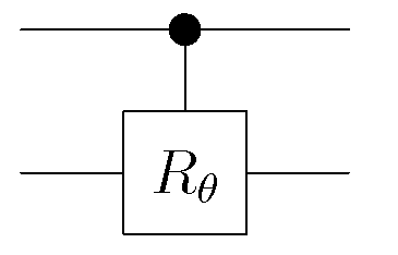
This is a two qubit controlled gate assuming that the control qubit is the most significant qubit, the action of this gate can be expressed as:

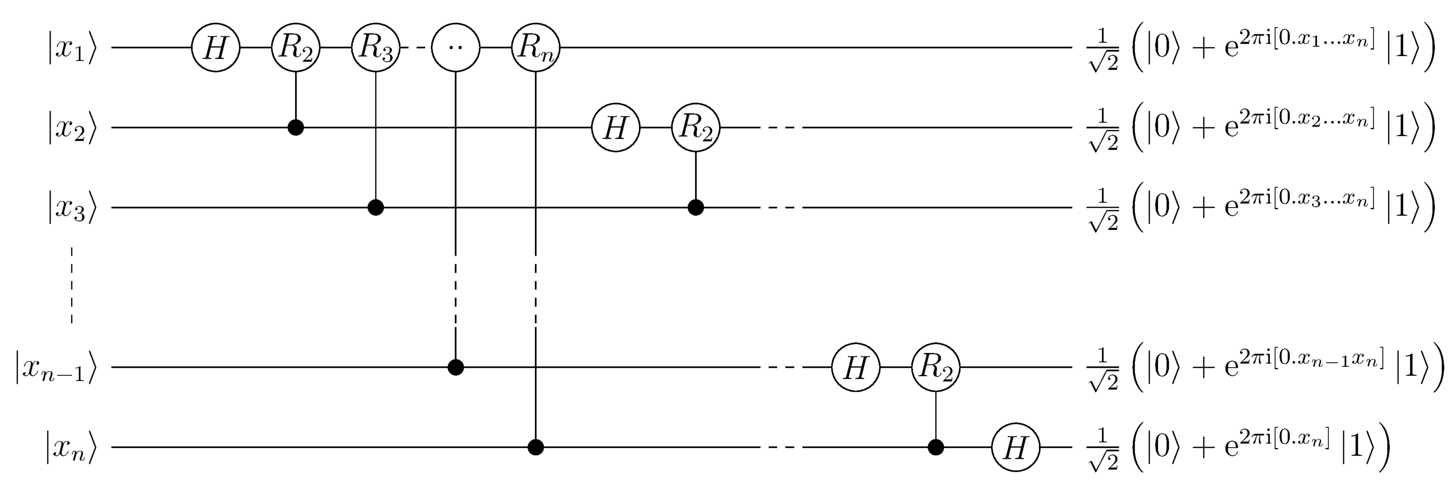
$\large R_{\theta}|0x\rangle = |0x\rangle$ $\large R_{\theta}|1x\rangle = e^{\frac{2\pi i}{2^{\theta}}}|1x\rangle$

Using these two gates, and the equation derived for QFT, we can construct the full circuit to get us the desired superposition like so

* Wikipedia

There’s a caveat here, the above circuit reverses the qubit order upside down, so many implementations swap the qubits to restore the qubit order. Depending on the application this swap may or may not be necessary. If you are having trouble understanding how does the circuit give us the needed superposition, I urge you to try writing it down for the case of 2 qubits. That’s what I did.

QFT circuit can be very easily made using Qiskit :

def qft_rotations(circuit, n):
    """Performs qft on the first n qubits in circuit (without swaps)"""
    if n == 0:
        return circuit
    n -= 1
    circuit.h(n)
    for qubit in range(n):
        circuit.cu1(pi/2**(n-qubit), qubit, n)
    #note the recursion
    qft_rotations(circuit, n)

def swap_registers(circuit, n):
    for qubit in range(n//2):
        circuit.swap(qubit, n-qubit-1)
    return circuit

def qft(circuit, n):
    """QFT on the first n qubits in circuit"""
    qft_rotations(circuit, n)
    swap_registers(circuit, n)
    return circuit

2. Representing Audio in quantum data

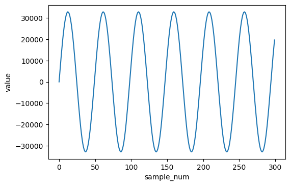
An audio file is simply a bunch of samples sampled at a specific sampling rate. Usually this rate is 44100Hz for CD quality audio. This means that the analog waveform is measured at 44100 equally spaced points within a second.

If we want to use QFT on such a wave we need to encode the value of each sample into the amplitudes of the basis states of our system. Consider this 3-qubit example:

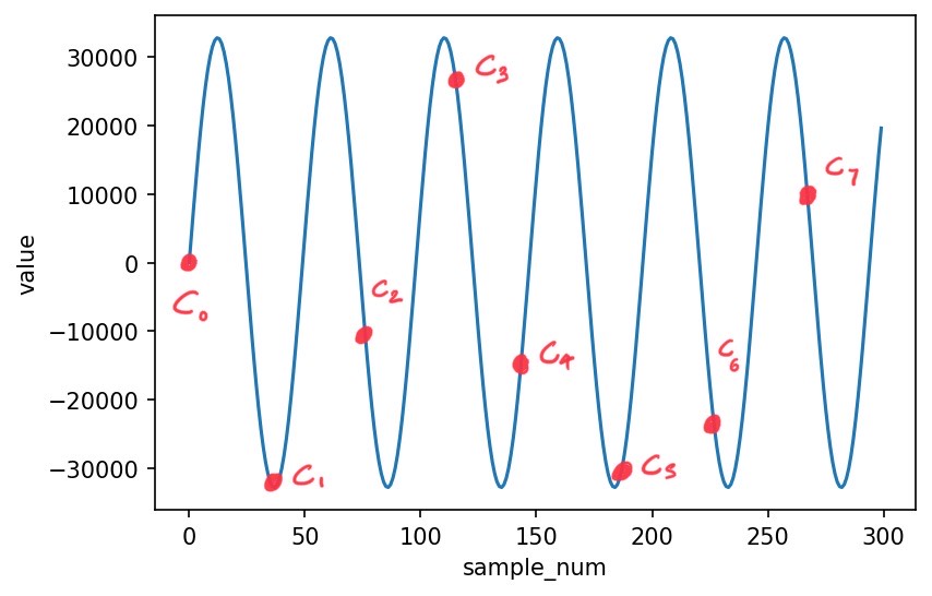
$\large |\psi_{audio}\rangle = c_{0}|000\rangle + c_{1}|001\rangle + c_{2}|010\rangle + c_{3}|011\rangle + c_{4}|100\rangle + c_{5}|101\rangle + c_{6}|110\rangle + c_{7}|111\rangle$

For a 3 qubit system, we can afford $2^{3}=8$ samples, which are denoted by the Cs in the above figure,

Note that Since $\psi_{audio}$ is a quantum state, we need

$\large \langle\psi_{audio}|\psi_{audio}\rangle = \sum_{i=0}^{7}|c_{i}|^{2} = 1$

Therefore, the Cs we sample need to be normalised before we can make a quantum state out of them.

3. Arbitrary state preparation

After getting all the Cs, its not trivial to put a system into the exact superposition that we want. To do that, you want to know what Schmidt decomposition is

3.1 Schmidt Decomposition Theorem

Any vector $\psi \in \mathcal{H}_{1} \otimes \mathcal{H}_{2}$ can be expressed in the form

$\large \psi = \sum_{j}c_{j}|\epsilon_{j}\rangle|\eta_{j}\rangle$

for non-negative real $c_{j}$ and orthonormal sets $\epsilon_{j}\in \mathcal{H}_{1}$ and $\eta_{j}\in \mathcal{H}_{2}$ . There are density operators $\rho_{1}$ on $\mathcal{H}_{1}$ and $\rho_{2}$ on $\mathcal{H}_{2}$ such that :

$\large \langle\psi|(A \otimes 1)|\psi \rangle = tr[A\rho_{1}]$ $\large \langle\psi|(1 \otimes B)|\psi \rangle = tr[A\rho_{2}]$

for all observables $A$ and $B$ on $\mathcal{H}_{1}$ and $\mathcal{H}_{2}$ respectively, and the $\{\epsilon_{j}\}$ can be chosen to be the eigenvectors of $\rho_{1}$ corresponding to the non-zero eigenvalues $p_{j}$ , the vectors $\{\eta_{j}\}$ , the corresponding eigenvectors for $\rho_{2}$ , and the positive scalars $c_{j} = \sqrt{p_{j}}$

3.2 State preparation

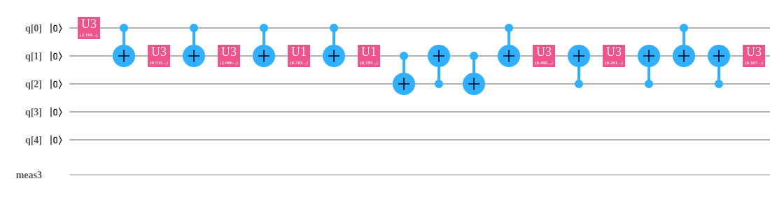
A general n-qubit state is fully described by $2^{n+1} - 2$ real parameters. These parameters are introduced sequentially in the form of C-NOT gates and single qubit rotation unitaries U. For example ,we can look at the process for a 4 qubit system below. For the general case I’d refer you to the paper “Quantum State Preparation with Universal Gate Decompositions”

In the case of four qubits, the Hilbert space can be factorized into two parts each of two qubits. An arbitrary pure state of four qubits can then be represented using the standard Schmidt decomposition as

$\large \psi = \sum_{i=1}^{4}\alpha_{i}|\psi\rangle_{i}|\phi\rangle_{i}$

After that the entire process can be broken down into four phases.

Phase 1

Starting with the initial state of all zeros, we generate the state with generalized schmidt coefficients on the first two qubits:

$\large |0000\rangle = (\alpha_{1}|00\rangle + \alpha_{2}|01\rangle + \alpha_{3}|10\rangle + \alpha_{4}|11\rangle)|00\rangle$

This can be done using a single C-NOT gate and single qubit rotations. For more details about this step refer “Decompositions of general quantum gates”

Phase 2

We perform two C-NOT operations, one with the control on the first qubit and the target on the third qubit and the other one with the control on the second qubit and the target on the fourth qubit. In such a way we can “copy” the basis states of the first two qubits onto the respective states of the second two qubits. In this way we obtain a state of four qubits, which has the same Schmidt decomposition coefficients as the target

$\large (\alpha_{1}|00\rangle + \alpha_{2}|01\rangle + \alpha_{3}|10\rangle + \alpha_{4}|11\rangle)|00\rangle \rightarrow (\alpha_{1}|00\rangle|00\rangle + \alpha_{2}|01\rangle|01\rangle + \alpha_{3}|10\rangle|10\rangle + \alpha_{4}|11\rangle|11\rangle)$

Phase 3

Keeping the Schmidt decomposition form we apply the unitary operation that transforms the basis states of the first two qubits into the four states, we obtain:

$\large |00\rangle \rightarrow |\psi\rangle_{1}$ $\large |01\rangle \rightarrow |\psi\rangle_{2}$ $\large |10\rangle \rightarrow |\psi\rangle_{3}$ $\large |11\rangle \rightarrow |\psi\rangle_{4}$

Phase 4

In the final phase of the circuit we perform a unitary operation on the third and fourth qubit in order to transform their computational basis states into the Schmidt basis states

$\large |00\rangle \rightarrow |\phi\rangle_{1}$ $\large |01\rangle \rightarrow |\phi\rangle_{2}$ $\large |10\rangle \rightarrow |\phi\rangle_{3}$ $\large |11\rangle \rightarrow |\phi\rangle_{4}$

This completes the state preparation.

3.3 State preparation in Qiskit

Thankfully, qiskit provides us with inbuilt functions for preparing arbitrary quantum states so we don’t have to do the above mathematical fuckery ourselves. Using Qiskit, a state preparer can be easily implemented using the following snippet of code:

def prepare_circuit(samples, normalize=True):

    """
    Args:
    amplitudes: List - A list of amplitudes with length equal to power of 2
    normalize: Bool - Optional flag to control normalization of samples, True by default
    Returns:
    circuit: QuantumCircuit - a quantum circuit initialized to the state given by amplitudes
    """
    num_amplitudes = len(samples)
    assert isPow2(num_amplitudes), 'len(amplitudes) should be power of 2'

    num_qubits = int(getlog2(num_amplitudes))
    q = QuantumRegister(num_qubits)
    qc = QuantumCircuit(q)

    if(normalize):
        ampls = samples / np.linalg.norm(samples)
    else:
        ampls = samples

    qc.initialize(ampls, [q[i] for i in range(num_qubits)])

    return qc

This is an example of how it looks, notice that it only uses C-NOT gates and single qubit rotations

Init Circuit

3.4 Important note

Given the noisy quantum processors that we currently have, its imperative to minimise the number of gates we have as much as possible. In my experience, in a 4-qubit IBM-Q system, as few as 50 gates was enough to introduce noise enough to get garbage output.

Hence, practically you might want to do your own optimizations to the state preparation circuit (e.g. getting rid of small angle rotations), which the qiskit inbuilt function does not allow.

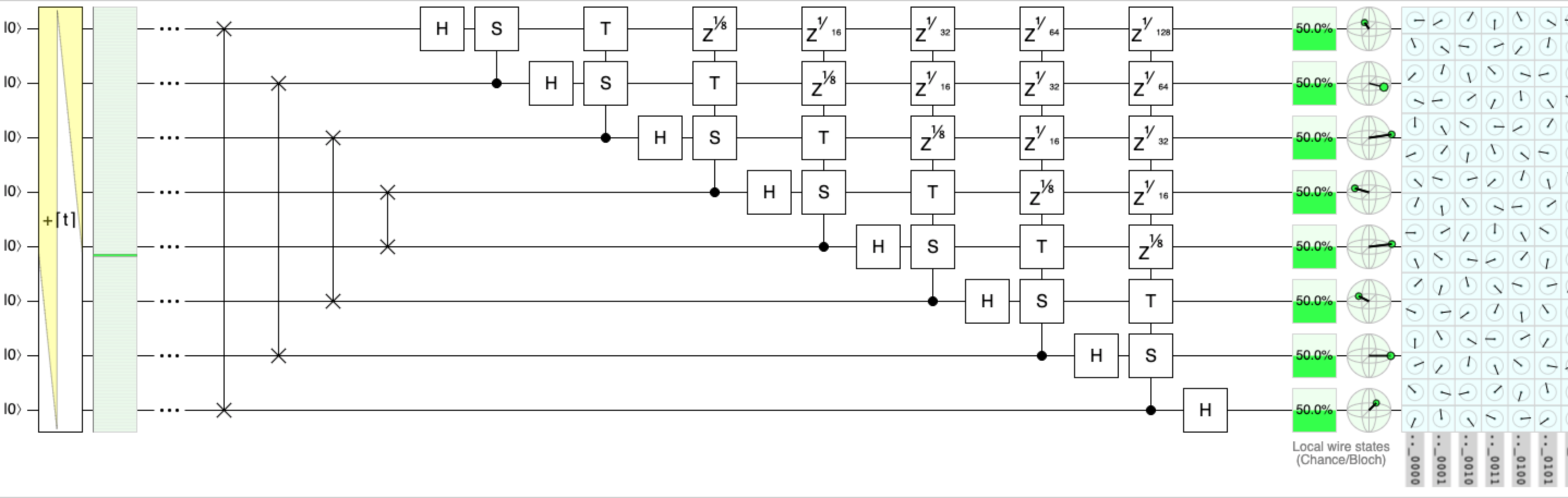
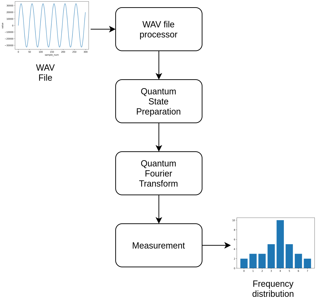
4. Running the experiment on a quantum simulator

Qiskit provides many simulator backend options, here I am going to use the qasm simulator backend, which mimics the behaviour of a noise-free real backend.

Since its a simulator, I am working with 16 qubits, which means I will be able to load in $2^{16} = 65536$ samples of my audio file.

The entire circuit can be split into 4 parts -

WAV file processor
Quantum state preparation
Quantum Fourier Transform
Measurement

I have used the pydub package to process the wav file. All quantum operations are done using Qiskit. The full code can be found in the linked github repository.

Pipeline

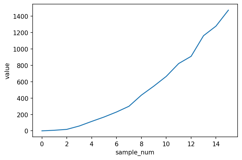
Step 1 - Input Audio file and prepare a quantum state

n_qubits = 16
audio = AudioSegment.from_file('900hz.wav')
samples = audio.get_array_of_samples()[:2**n_qubits]
plt.xlabel('sample_num')
plt.ylabel('value')
plt.plot(list(range(len(samples))), samples)

# prepare circuit
qcs = prepare_circuit_from_samples(samples, n_qubits)

Step 2 - Apply QFT and get amplitudes in the fourier space

qcs = prepare_circuit_from_samples(samples, n_qubits)
qft(qcs, n_qubits)
qcs.measure_all()

qasm_backend = Aer.get_backend('qasm_simulator')
out = execute(qcs, qasm_backend, shots=8192).result()

Step 3 - Measurement

When a quantum circuit is run, at the end each qubit is measured in the Pauli-Z basis. Hence, all the qubits collapse into one of the two eigenstates of the Pauli-Z operator. But they do so with the probabilities dictated by the superposition that we put the qubits in. The big mathematical fuckery that we did in section 1 was precisely to get each qubit in a superposition that would make the qubits collapse in a way that gives us the fourier transform of the input amplitudes.

If the final output of the state is given by :

$\large |\psi\rangle = \sum_{i}c_{i}|i\rangle$

where $i$ are the basis states, then the information we need is in the $c_{i}$

However since we can only observe the distribution of the final qubits, we can only measure $\|c_{i}\|^{2}$

To get this distribution we run the circuit many times, which is controlled by the shots parameter.

After measurement, we still need to convert the distribution that we get into actual frequencies. This is a pretty standard operation on discrete fourier transforms. If you feel uncomfortable understanding the next few lines I’d suggest you see the discrete fourier transform page on wikipedia.

out = execute(qcs, qasm_backend, shots=8192).result()
counts = out.get_counts()
fft = get_fft_from_counts(counts, n_qubits)[:n_samples//2]
plot_samples(fft[:2000])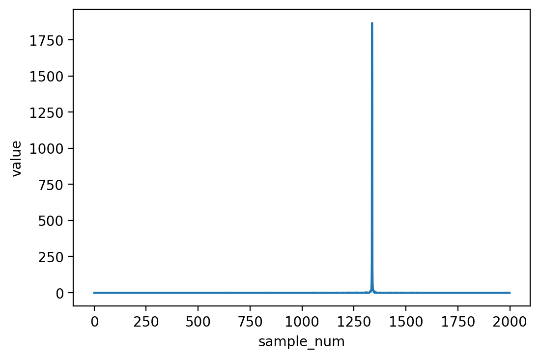

f-space

We see a nice peak at about 1300. To get the value of frequency we have to multiply this peak by $\frac{frame\_rate}{n\_samples}$ . Note that we can only measure upto $\frac{frame\_rate}{2}Hz$ - which is the Nyquist limit. If you don’t know what that means google is your friend.

top_indices = np.argsort(-np.array(fft))
freqs = top_indices*frame_rate/n_samples
# get top 5 detected frequencies
freqs[:5]
=> Prints out: array([899.68414307, 900.35705566, 899.01123047, 901.02996826,
       898.33831787])

Nice! Great Success

Running the experiment on real quantum hardware!

Totally different beast that is. Real quantum hardware that we currently have is extremely noisy.

The way you access real quantum hardware is by making use of IBM - Q Experience. Currently it offers various real quantum backends. One of the backends has a capacity of 16 qubits (ibmq_16_melbourne), while the rest have only 5 qubits

Trial 1

I tried the circuit that I built in the previous sections as is on the 16 qubit backend - it failed.

No surprises there, I was sure it couldn’t be that easy. The problem was that I was exceeding the max depth (number of gates) allowed by the backend.

error1

Result: Failure

Trial 2

I figured perhaps the 16 qubit experiment is a bit too much, so I tried simplifying it to 5 qubits, with a very low sample size of $2^5 = 32$ samples. With such a small number of samples, to get a decent frequency resolution, I had to drastically decrease the sampling rate to $2000$ , which gave a frequency resolution of

$\delta f = \frac{sampling\_rate}{n\_samples} = \frac{2000}{32} = 62.5$

I first ran the experiment on the qasm_simulator to see how the desired output should look like:

n_qubits = 5
n_samples = 2**n_qubits
audio = AudioSegment.from_file('900hz.wav')
audio = audio.set_frame_rate(2000)
frame_rate = audio.frame_rate #2000
samples = audio.get_array_of_samples()[:n_samples]
plt.xlabel('sample_num')
plt.ylabel('value')
plt.plot(list(range(len(samples))), samples)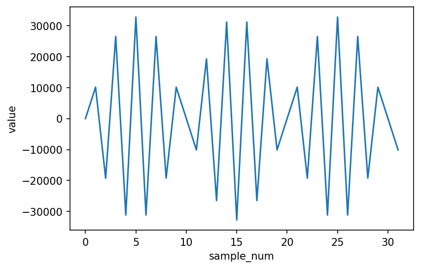

sine_900_2000

With so few samples, the plot starts loosing its sine-wavy looks.

qcs = prepare_circuit_from_samples(samples, n_qubits)
qft(qcs, n_qubits)
qcs.measure_all()

qasm_backend = Aer.get_backend('qasm_simulator')
out = execute(qcs, qasm_backend, shots=8192).result()
counts = out.get_counts()
fft = get_fft_from_counts(counts, n_qubits)[:n_samples//2]


plt.xlabel('sample_num')
plt.ylabel('value')
plt.plot(list(range(len(fft[:]))), fft[:])

top_indices = np.argsort(-np.array(fft))
freqs = top_indices*frame_rate/n_samples
# get top 5 detected frequencies
freqs[:5]
=> Prints: array([875. , 937.5, 812.5, 750. , 687.5])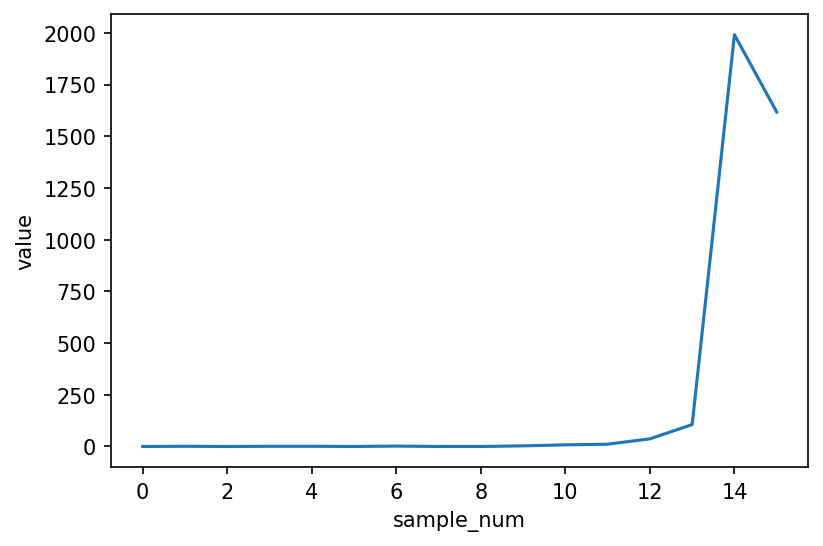

f32

The plot makes sense with one strong peak. Alright lets get real and try it on real hardware.

provider = IBMQ.get_provider(hub='ibm-q')
backend = least_busy(provider.backends(filters=lambda x: x.configuration().n_qubits >= n_qubits
                                       and not x.configuration().simulator
                                       and x.status().operational==True))
print("least busy backend: ", backend)
=> least busy backend:  ibmqx2
out = execute(qcs, qasm_backend, shots=8192).result()

You can see the results of your experiments in the IBM Q Experience portal. For this particular experiment, it showed me this:

ibmq_32

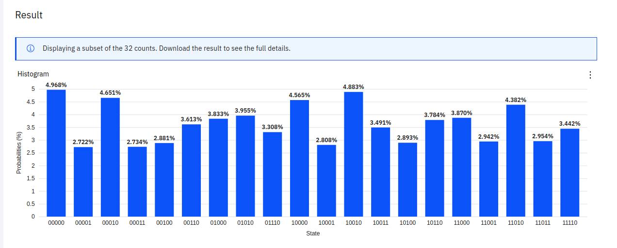
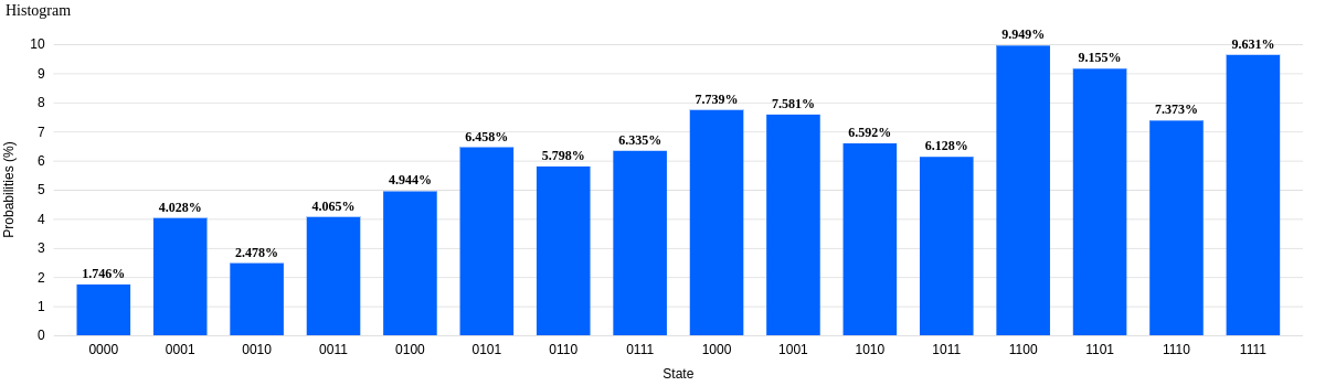
Which is gibberish, we ideally should get one single peak. So something’s clearly wrong.

Result: Failure

Trial 3

I thought maybe there is something wrong in the way the state is prepared from the audio file. This was supported by the fact that more than half of the gates in the circuit were actually used for state preparation.

I reduced the number of qubits to 4, and created a dummy state comprising of basis states with linearly increasing amplitudes.

n_qubits = 4
dummy_state = [i for i in range(2**n_qubits)]
=> dummy_state = [0, 1, 2, 3, 4, 5, 6, 7, 8, 9, 10, 11, 12, 13, 14, 15]

qcs = prepare_circuit_from_samples(dummy_state, n_qubits, normalize=True)
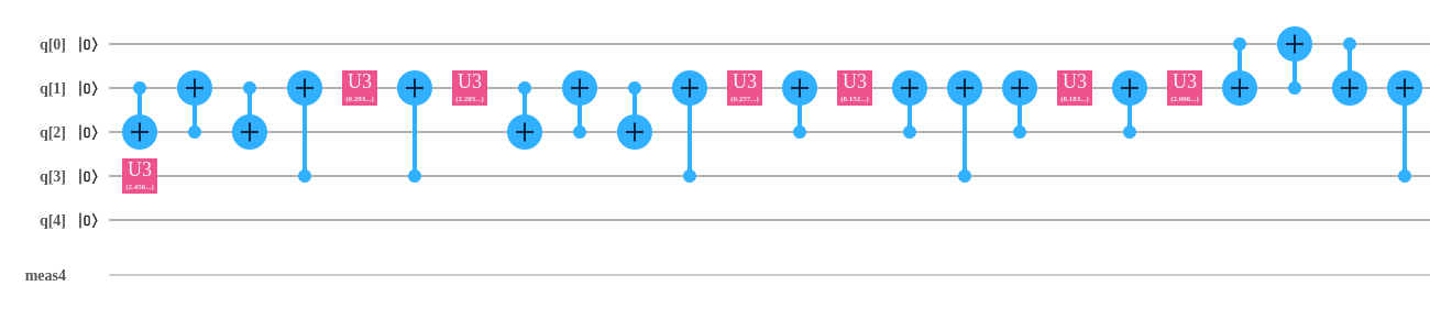
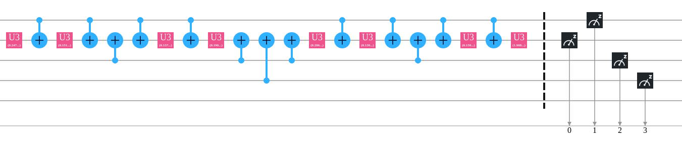
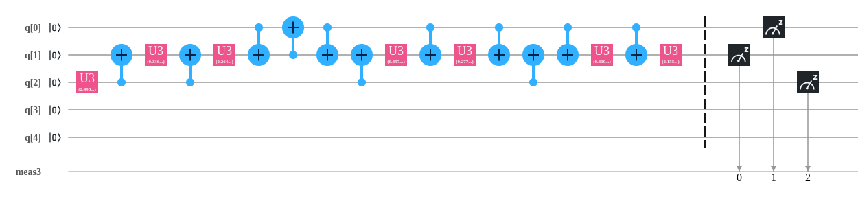
qcs.measure_all()

The circuit as visualized on IBM Q portal:

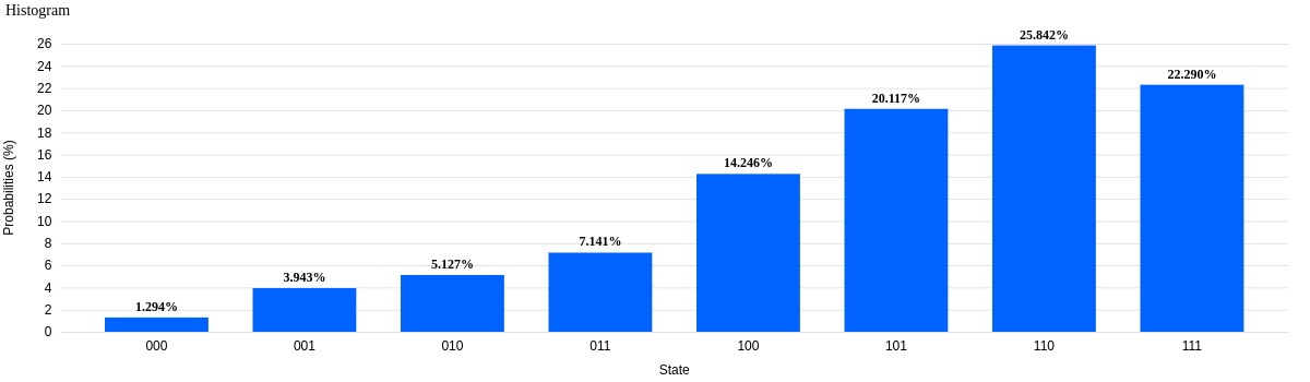
After running on a simulator, the results look like :

f_16

Which looks good as expected.

After running it on real hardware:

Its noisy again! borderline gibberish. Ideally the amplitudes should go up linearly. But at least the problem has been isolated.

Lets try the same dummy state preparation with 3 qubits.

n_qubits = 3
dummy_state = [i for i in range(2**n_qubits)]
=> dummy_state = [0, 1, 2, 3, 4, 5, 6, 7]

qcs = prepare_circuit_from_samples(dummy_state, n_qubits, normalize=True)
qcs.measure_all()

The circuit as visualized on IBM Q portal:

After running on a simulator, the results look like :

f_16

Which looks good as expected.

After running it on real hardware:

Now we are talking! This looks much more acceptable than previous experiments. Which sadly means that we will have to restrict ourselves a a meagre 3 qubits, which is only 8 samples. Lets see what we can do with it.

Result: almost Success

Trial 4

Running the entire circuit, with a sampling rate of $2000$ , and only 3 qubits

n_qubits = 3
n_samples = 2**n_qubits
audio = AudioSegment.from_file('900hz.wav')
audio = audio.set_frame_rate(2000)
frame_rate = audio.frame_rate #2000
samples = audio.get_array_of_samples()[:n_samples]

qcs = prepare_circuit_from_samples(samples, n_qubits)
qft(qcs, n_qubits)
qcs.measure_all()

provider = IBMQ.get_provider(hub='ibm-q')
backend = least_busy(provider.backends(filters=lambda x: x.configuration().n_qubits >= n_qubits
                                       and not x.configuration().simulator
                                       and x.status().operational==True))
print("least busy backend: ", backend)
=> least busy backend:  ibmqx2
out = execute(qcs, qasm_backend, shots=8192).result()

The result looks like:

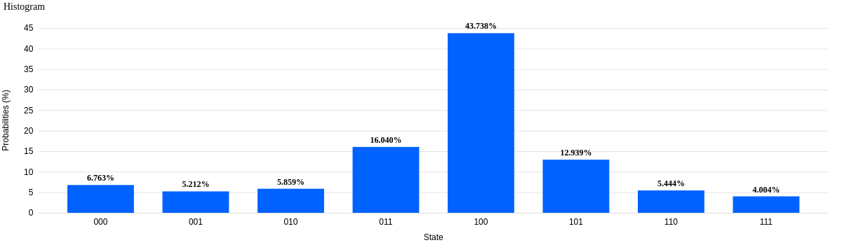
Nice! we see a clear peak. The peak seems to be at $100$ which is $4$ . To get the associated frequency :

$\delta f = \frac{2000}{8} = 250Hz$ $F = 4 * \frac{sampling\_rate}{n\_samples} = 4 * \frac{2000}{8} \pm \delta f$ $= 1000 \pm 250Hz$

Nice!

Result: Success! (?)

I gotta say..

This work is more like a proof of concept. It may not look like much for now but as we move towards fault tolerant, less error prone quantum hardware, our capacities would increase exponentially.

There could be a lot of ways in which this work can be improved even with the current hardware. For starters:

No error correction was used.
Approximate quantum fourier transform could’ve been used, where we get rid of small angle rotations to minimize the number of gates.
State preparation routine could be made approximate to further minimize number of gates.

Quantum Computing to find frequencies in an audio file

Because why not...